import numpy as np
import matplotlib.pyplot as plt

np.random.seed(45)

%matplotlib inline

Linear Regression using Normal Equation

Closed-form equation for minimizing the cost function for Linear Regression. Writing math in markdown

temp = $X^T$ * $X$

$\theta$ = $($temp$)^{-1}$ $X^T$ $y$

# Generating data for this equation
X = np.random.rand(100, 1)
y = 4 + 3 * X + np.random.randn(100, 1)

Now let’s compute θ using the Normal Equation. We will use the inv() function from NumPy’s Linear Algebra module (np.linalg) to compute the inverse of a matrix, andthe dot() method for matrix multiplication:

X_b = np.c_[np.ones((100, 1)), X] # add x0=1 to each instance
theta_best = np.linalg.inv(X_b.T.dot(X_b)).dot(X_b.T).dot(y)

The actual function that we used to generate the data is y = 4 + 3x0 + Gaussian noise. Let’s see what the equation found:

theta_best

array([[4.1130839 ],
       [2.84220224]])

Now you can make predictions using θ:

X_new = np.array([[0], [2]])
X_new_b = np.c_[np.ones((2, 1)), X_new] 
y_predict = X_new_b.dot(theta_best)
y_predict

array([[4.1130839 ],
       [9.79748838]])

Plotting the models predictions

plt.plot(X_new, y_predict, "r-")
plt.plot(X, y, "b.")
plt.axis([0, 2, 0, 15])
plt.show()

# We can do the same using sklearn
from sklearn.linear_model import LinearRegression
lin_reg = LinearRegression()
lin_reg.fit(X, y)
print(lin_reg.intercept_, lin_reg.coef_)
lin_reg.predict(X_new)

[4.1130839] [[2.84220224]]

array([[4.1130839 ],
       [9.79748838]])

Gradient Descent

Another way to train Linear Regression Model - Gradient Descent

The general idea of Gradient Descent is totweak parameters iteratively in order to minimize a cost function.

Why Gradient Descent always works for Linear Regression?: Because of the cost function(MSE-mean squared error). MSE cost function for a Linear Regression model happens to be aconvex function, which means that if you pick any two points on the curve, the linesegment joining them never crosses the curve. This implies that there are no localminima, just one global minimum. It is also a continuous function with a slope thatnever changes abruptly. These two facts have a great consequence: Gradient Descentis guaranteed to approach arbitrarily close the global minimum (if you wait longenough and if the learning rate is not too high).

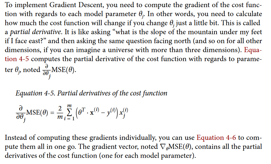
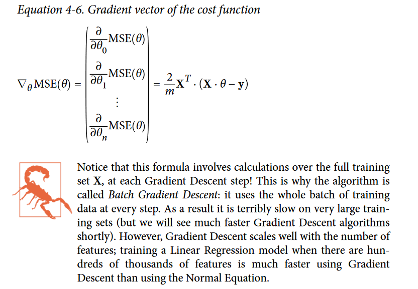
Once you have the gradient vector, which points uphill, just go in the opposite direction to go downhill. This means subtracting ∇_θMSE(θ) from θ. This is where the learning rate η comes into play: multiply the gradient vector by η to determine thesize of the downhill step.

θ = θ − η*(∇_θMSE(θ))

eta = 0.1 # learning reate
n_iterations = 1000
m = 100 # number of training examples

theta = np.random.randn(2, 1) # random initialization

for iteration in range(n_iterations):
    gradients = 2/m*X_b.T.dot(X_b.dot(theta) - y)
    theta = theta - eta*gradients

print(theta)

[[4.11308449]
 [2.84220113]]

This is exactly what the normal equation found!

Stochastic Gradient Descent

• The main problem with Batch Gradient Descent is the fact that it uses the wholetraining set to compute the gradients at every step, which makes it very slow whenthe training set is large.
• At the opposite extreme, Stochastic Gradient Descent just picks a random instance in the training set at every step and computes the gradientsbased only on that single instance.
• Obviously this makes the algorithm much fastersince it has very little data to manipulate at every iteration. It also makes it possible totrain on huge training sets, since only one instance needs to be in memory at eachiteration (SGD can be implemented as an out-of-core algorithm.)
• Over time it will end up very close to the minimum, but once it gets there it willcontinue to bounce around, never settling down. So once the algo‐rithm stops, the final parameter values are good, but not optimal.
• When the cost function is very irregular, this can actually help the algorithm jump out of local minima, so Stochastic Gradient Descent has a betterchance of finding the global minimum than Batch Gradient Descent does.
• Therefore randomness is good to escape from local optima, but bad because it meansthat the algorithm can never settle at the minimum.
  • One solution to this dilemma isto gradually reduce the learning rate. The steps start out large (which helps makequick progress and escape local minima), then get smaller and smaller, allowing thealgorithm to settle at the global minimum. This process is called simulated annealing.
  • The function that determines the learning rate at each iterationis called the learning schedule. If the learning rate is reduced too quickly, you may getstuck in a local minimum, or even end up frozen halfway to the minimum. If thelearning rate is reduced too slowly, you may jump around the minimum for a longtime and end up with a suboptimal solution if you halt training too early.

# SGD using a simple learning schedule
n_epochs = 50
t0, t1 = 5, 50 # learning schedule hyperparameter

def learning_schedule(t):
    return t0/(t+t1)

theta = np.random.randn(2, 1) # random initialization

for epoch in range(n_epochs):
    for i in range(m):
        random_index = np.random.randint(m)
        xi = X_b[random_index:random_index+1]
        yi = y[random_index:random_index+1]
        gradients = 2*xi.T.dot(xi.dot(theta)-yi) # do not use 2/m as here only one training example
        eta = learning_schedule(epoch*m + i)
        theta = theta - eta*gradients

print(theta)

[[4.15137068]
 [2.80929092]]

By convention we iterate by rounds of m iterations; each round is called an epoch. While the Batch Gradient Descent code iterated 1,000 times through the whole training set, this code goes through the training set only 50 times and reaches a fairly good solution

To perform Linear Regression using SGD with Scikit-Learn, you can use the SGDRegressor class, which defaults to optimizing the squared error cost function. The following code runs 50 epochs, starting with a learning rate of 0.1 (eta0=0.1), using the default learning schedule (different from the preceding one), and it does not use any regularization (penalty=None; more details on this shortly):

from sklearn.linear_model import SGDRegressor
sgd_reg = SGDRegressor(max_iter=50, penalty=None, eta0=0.1)
sgd_reg.fit(X, y.ravel())

print(sgd_reg.intercept_, sgd_reg.coef_)

[4.163805] [2.78003544]

Mini-batch Gradient Descent

• It is quite simple to understand once you know Batch and Stochastic Gradi‐ent Descent: at each step, instead of computing the gradients based on the full training set (as in Batch GD) or based on just one instance (as in Stochastic GD), Mini-batch GD computes the gradients on small random sets of instances called mini-batches.

Polynomial Regression

• What if your data is actually more complex than a simple straight line? Surprisingly, you can actually use a linear model to fit nonlinear data. A simple way to do this is to add powers of each feature as new features, then train a linear model on this extendedset of features. This technique is called Polynomial Regression.

Let’s generate some nonlinear data, based on a simple quadratic equation(with some noise)

m = 100
X = 6*np.random.rand(m, 1) - 3
y = 0.5 * X**2 + X + 2 + np.random.randn(m, 1)

y = (0.5)x² + x + c

# visualising this data
plt.plot(X, y, "b.")
plt.xlabel('X')
plt.ylabel('y')
plt.axis([-3, 3, 0, 10])
plt.show()

Clearly, a straight line will never fit this data properly. So let’s use Scikit-Learn’s PolynomialFeatures class to transform our training data, adding the square (2nd-degree polynomial) of each feature in the training set as new features (in this case there is just one feature):

PolynomialFeatures: Generate a new feature matrix consisting of all polynomial combinations of the features with degree less than or equal to the specified degree. For example, if an input sample is two dimensional and of the form [a, b], the degree-2 polynomial features are [1, a, b, a^2, ab, b^2].

https://scikit-learn.org/stable/modules/generated/sklearn.preprocessing.PolynomialFeatures.html

from sklearn.preprocessing import PolynomialFeatures
poly_features = PolynomialFeatures(degree=2, include_bias=False)
X_poly = poly_features.fit_transform(X)
print('X[0]=', X[0])
print('X_poly[0]=', X_poly[0])

X[0]= [-0.49180502]
X_poly[0]= [-0.49180502  0.24187218]

X_poly now contains the original feature of X plus the square of this feature. Now you can fit a LinearRegression model to this extended training data

lin_reg = LinearRegression()
lin_reg.fit(X_poly, y)
print(lin_reg.intercept_, lin_reg.coef_)

[2.10246792] [[0.96070033 0.54007905]]

X_new=np.linspace(-3, 3, 100).reshape(100, 1)
X_new_poly = poly_features.transform(X_new)
y_new = lin_reg.predict(X_new_poly)
plt.plot(X, y, "b.")
plt.plot(X_new, y_new, "r-", linewidth=2, label="Predictions")
plt.plot()
plt.xlabel('X')
plt.ylabel('y')
plt.axis([-3, 3, 0, 10])
plt.show()

Note that when there are multiple features, Polynomial Regression is capable of find‐ing relationships between features (which is something a plain Linear Regressionmodel cannot do). This is made possible by the fact that PolynomialFeatures alsoadds all combinations of features up to the given degree. For example, if there were two features a and b, PolynomialFeatures with degree=3 would not only add the features a², a³, b², and b³, but also the combinations ab, a²b, and ab².

How to tell if a model is too simple or too complex?

• If a model performs well on the training data but generalizes poorly according to the cross-validation metrics, then your model is overfitting. If it performs poorly on both, then it is underfitting. This is one way to tell when a model is too simple or too complex.
• Another way is to look at the learning curves: these are plots of the model’s performance on the training set and the validation set as a function of the training set size.
• To generate the plots, simply train the model several times on different sized subsets of the training set.
• IMPORTANT:
  • high bias = underfitiing
  • high variance = overfitting

# The  following  code  defines  a  function  that  plots  the  learningcurves of a model given some training data:
from sklearn.metrics import mean_squared_error
from sklearn.model_selection import train_test_split
from sklearn.linear_model import LinearRegression

np.random.seed(31)
X = np.random.rand(100, 1)
y = 4 + 3 * X + np.random.randn(100, 1)

def plot_learning_curve(model, X, y):
    X_train, X_val, y_train, y_val = train_test_split(X, y, test_size=0.2)
    train_errors, val_errors = [], []
    for m in range(1, len(X_train)):
        model.fit(X_train[:m], y_train[:m])
        y_train_predict = model.predict(X_train[:m])
        y_val_predict = model.predict(X_val)
        train_errors.append(mean_squared_error(y_train_predict, y_train[:m]))
        val_errors.append(mean_squared_error(y_val_predict, y_val))
    plt.xlabel('Training Set Size')
    plt.ylabel('RMSE')
    plt.plot(np.sqrt(train_errors), "r-+", linewidth=2, label="train") #training error
    plt.plot(np.sqrt(val_errors), "b-", linewidth=3, label="val") # validation error

# learning curve for linear regression
lin_reg = LinearRegression()
plot_learning_curve(lin_reg, X, y)

• First, let’s look at the performance on the trainingdata: when there are just one or two instances in the training set, the model can fit them perfectly, which is why the curve starts at zero. But as new instances are added to the training set, it becomes impossible for the model to fit the training data perfectly, both because the data is noisy and because it is not linear at all. So the error onthe training data goes up until it reaches a plateau, at which point adding new instances to the training set doesn’t make the average error much better or worse.
• Now let’slook at the performance of the model on the validation data. When the model is trained on very few training instances, it is incapable of generalizing properly, which is why the validation error is initially quite big. Then as the model is shown more training examples, it learns and thus the validation error slowly goes down. However,once again a straight line cannot do a good job modeling the data, so the error ends up at a plateau, very close to the other curve.
• These learning curves(the one above) are typical of an underfitting model.
• Now let’s look at the learning curves of a 10th-degree polynomial model on the same data

from sklearn.pipeline import Pipeline

np.random.seed(31)

X = np.random.rand(100, 1)
y = 4 + 3 * X + np.random.randn(100, 1)

polynomial_regression = Pipeline((
    ("poly_features", PolynomialFeatures(degree=10, include_bias=False)),
    ("sgd_reg", LinearRegression()),
))

plt.axis([0, 80, 0, 3])
plot_learning_curve(polynomial_regression, X, y)

NOTE: This diagram is not very clear

• The error on the training data is much lower than with the Linear Regressionmodel.
• There is a gap between the curves. This means that the model performs significantly better on the training data than on the validation data, which is the hall mark of an overfitting model. However, if you used a much larger training set,the two curves would continue to get closer.
• One way to improve an overfitting model is to feed it more training data until the validation error reaches the training error.

Regularized Linear Models

Ridge Regression

• Ridge Regression (also called Tikhonov regularization) is a regularized version of Linear Regression
• A regularization term equal to $α$ $∑_{i=1}^n$ = $θ_i^2$ is added to the cost function.
• This forces the learning algorithm to not only fit the data but also keep the model weights as small as possible.
• Note that the regularization term should only be added to the cost function during training. Once the model is trained, you want to evaluate the model’s performance using the unregularized performance measure.
• The hyperparameter α controls how much you want to regularize the model. If α = 0 then Ridge Regression is just Linear Regression.
• If α is very large, then there will be bias(underfitting)

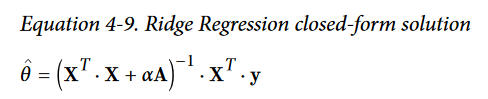
• Here is the closed form solution for Ridge Regression

• The regularization term is half the square of the ℓ₂ norm

from sklearn.linear_model import Ridge
from sklearn.preprocessing import StandardScaler

np.random.seed(42)
m = 20
X = 3 * np.random.rand(m, 1)
y = 1 + 0.5 * X + np.random.randn(m, 1) / 1.5
X_new = np.linspace(0, 3, 100).reshape(100, 1)

def plot_model(model_class, polynomial, alphas, **model_kargs):
    for alpha, style in zip(alphas, ("b-", "g--", "r:")):
        model = model_class(alpha, **model_kargs) if alpha > 0 else LinearRegression()
        if polynomial:
            model = Pipeline([
                    ("poly_features", PolynomialFeatures(degree=10, include_bias=False)),
                    ("std_scaler", StandardScaler()),
                    ("regul_reg", model),
                ])
        model.fit(X, y)
        y_new_regul = model.predict(X_new)
        lw = 2 if alpha > 0 else 1
        plt.plot(X_new, y_new_regul, style, linewidth=lw, label=r"$\alpha = {}$".format(alpha))
    plt.plot(X, y, "b.", linewidth=3)
    plt.legend(loc="upper left", fontsize=15)
    plt.xlabel("$x_1$", fontsize=18)
    plt.axis([0, 3, 0, 4])

plt.figure(figsize=(8,4))
plt.subplot(121)
plot_model(Ridge, polynomial=False, alphas=(0, 10, 100), random_state=42)
plt.ylabel("$y$", rotation=0, fontsize=18)
plt.subplot(122)
plot_model(Ridge, polynomial=True, alphas=(0, 10**-5, 1), random_state=42)


plt.show()

# Ridge Regression using sklearn
from sklearn.linear_model import Ridge
ridge_reg = Ridge(alpha=1, solver="cholesky", random_state=42)
ridge_reg.fit(X, y) # uses the X, y defined in the above cell
ridge_reg.predict([[1.5]])

array([[1.55071465]])

# using SGD
sgd_reg = SGDRegressor(max_iter=50, tol=-np.infty, penalty="l2", random_state=42)
sgd_reg.fit(X, y.ravel())
sgd_reg.predict([[1.5]])

array([1.49905184])

The penalty hyperparameter sets the type of regularization term to use. Specifying"l2" indicates that you want SGD to add a regularization term to the cost function equal to half the square of the ℓ2 norm of the weight vector: this is simply RidgeRegression.

ridge_reg = Ridge(alpha=1, solver="sag", random_state=42)
ridge_reg.fit(X, y)
ridge_reg.predict([[1.5]])

array([[1.5507201]])

Lasso Regression

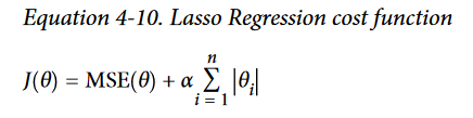
• Least Absolute Shrinkage and Selection Operator Regression (simply called Lasso Regression) is another regularized version of Linear Regression: just like Ridge Regression, it adds a regularization term to the cost function, but it uses the ℓ₁ norm of the weight vector instead of half the square of the ℓ₂ norm
• An important characteristic of Lasso Regression is that it tends to completely eliminate the weights of the least important features (i.e., set them to zero).
• Here is a small Scikit-Learn example using the Lasso class. Note that you could instead use an SGDRegressor(penalty="l1").

from sklearn.linear_model import Lasso

lasso_reg = Lasso(alpha=0.1)
lasso_reg.fit(X, y)
lasso_reg.predict([[1.5]])

array([1.53788174])

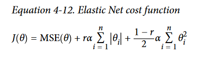
Elastic Net

• Elastic Net is a middle ground between Ridge Regression and Lasso Regression.
• The regularization term is a simple mix of both Ridge and Lasso’s regularization terms, and you can control the mix ratio r. When r = 0, Elastic Net is equivalent to Ridge Regression, and when r = 1, it is equivalent to Lasso Regression
• So when should you use Linear Regression, Ridge, Lasso, or Elastic Net?
• It is almost always preferable to have at least a little bit of regularization, so generally you should avoid plain Linear Regression.
• Ridge is a good default, but if you suspect that only a few features are actually useful, you should prefer Lasso or Elastic Net since they tend to reduce the useless features’ weights down to zero as we have discussed.
• In general, Elastic Net is preferred over Lasso since Lasso may behave erratically when the number of features is greater than the number of training instances or when several features are strongly correlated.
• Here is a short example using Scikit-Learn’s ElasticNet (l1_ratio corresponds tothe mix ratio r):

from sklearn.linear_model import ElasticNet
elastic_net = ElasticNet(alpha=0.1, l1_ratio=0.5, random_state=42)
elastic_net.fit(X, y)
elastic_net.predict([[1.5]])

array([1.54333232])

Early Stopping

• A very different way to regularize iterative learning algorithms such as GradientDescent is to stop training as soon as the validation error reaches a minimum. This iscalled early stopping.

Logistic Regression

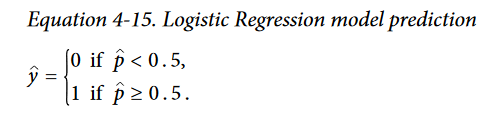
• Logistic regression is a binary classifier. If the estimated probability is greater than 50% the model predicts that particular instance belonging to class 1, else class 0
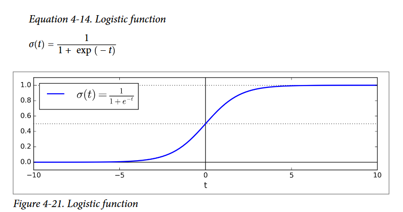
• Just like a Linear Regression model, a Logistic Regression model computes a weighted sum of the input features (plus a bias term), but instead of outputting the result directly like the Linear Regression model does, it outputs the logistic of this result
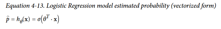
• Once the Logistic Regression model has estimated the probability p = hθ(x) that an instance x belongs to the positive class, it can make its prediction ŷ easily
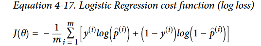
• Cost Function for Logistic Regression
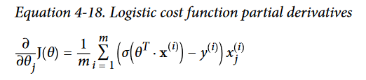
• Logistic Regression partial derivative

# Logistic Regression using the iris classification example
from sklearn import datasets
iris = datasets.load_iris()
list(iris.keys())

X = iris['data'][:, 3: ] # petal width
y = (iris['target']==2).astype(np.int) # 1 if Iris-Virginica, else 0

# Now let’s train a Logistic Regression model:
from sklearn.linear_model import LogisticRegression

log_reg = LogisticRegression()
log_reg.fit(X, y)

# Let’s look at the model’s estimated probabilities for flowers with petal widths varyingfrom 0 to 3 cm
X_new = np.linspace(0, 3, 1000).reshape(-1, 1)
y_proba = log_reg.predict_proba(X_new)
plt.plot(X_new, y_proba[:, 1], "g-", label="Iris-Virginica")
plt.plot(X_new, y_proba[:, 0], "b--", label="Not Iris-Virginica")

[<matplotlib.lines.Line2D at 0x1673da43b88>]

# A fancier plot
X_new = np.linspace(0, 3, 1000).reshape(-1, 1)
y_proba = log_reg.predict_proba(X_new)
decision_boundary = X_new[y_proba[:, 1] >= 0.5][0]

plt.figure(figsize=(8, 3))
plt.plot(X[y==0], y[y==0], "bs")
plt.plot(X[y==1], y[y==1], "g^")
plt.plot([decision_boundary, decision_boundary], [-1, 2], "k:", linewidth=2)
plt.plot(X_new, y_proba[:, 1], "g-", linewidth=2, label="Iris-Virginica")
plt.plot(X_new, y_proba[:, 0], "b--", linewidth=2, label="Not Iris-Virginica")
plt.text(decision_boundary+0.02, 0.15, "Decision  boundary", fontsize=14, color="k", ha="center")
plt.arrow(decision_boundary, 0.08, -0.3, 0, head_width=0.05, head_length=0.1, fc='b', ec='b')
plt.arrow(decision_boundary, 0.92, 0.3, 0, head_width=0.05, head_length=0.1, fc='g', ec='g')
plt.xlabel("Petal width (cm)", fontsize=14)
plt.ylabel("Probability", fontsize=14)
plt.legend(loc="center left", fontsize=14)
plt.axis([0, 3, -0.02, 1.02])
plt.show()

from sklearn.linear_model import LogisticRegression

X = iris["data"][:, (2, 3)]  # petal length, petal width
y = (iris["target"] == 2).astype(np.int)

log_reg = LogisticRegression(solver="liblinear", C=10**10, random_state=42)
log_reg.fit(X, y)

x0, x1 = np.meshgrid(
        np.linspace(2.9, 7, 500).reshape(-1, 1),
        np.linspace(0.8, 2.7, 200).reshape(-1, 1),
    )
X_new = np.c_[x0.ravel(), x1.ravel()]

y_proba = log_reg.predict_proba(X_new)

plt.figure(figsize=(10, 4))
plt.plot(X[y==0, 0], X[y==0, 1], "bs")
plt.plot(X[y==1, 0], X[y==1, 1], "g^")

zz = y_proba[:, 1].reshape(x0.shape)
contour = plt.contour(x0, x1, zz, cmap=plt.cm.brg)


left_right = np.array([2.9, 7])
boundary = -(log_reg.coef_[0][0] * left_right + log_reg.intercept_[0]) / log_reg.coef_[0][1]

plt.clabel(contour, inline=1, fontsize=12)
plt.plot(left_right, boundary, "k--", linewidth=3)
plt.text(3.5, 1.5, "Not Iris-Virginica", fontsize=14, color="b", ha="center")
plt.text(6.5, 2.3, "Iris-Virginica", fontsize=14, color="g", ha="center")
plt.xlabel("Petal length", fontsize=14)
plt.ylabel("Petal width", fontsize=14)
plt.axis([2.9, 7, 0.8, 2.7])
plt.show()

Softmax Regression

• The Logistic Regression model can be generalized to support multiple classes directly, without having to train and combine multiple binary classifiers
• This is called Softmax Regression, or Multinomial Logistic Regression
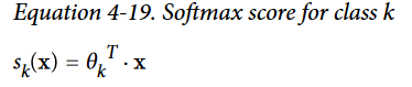
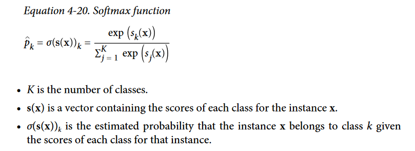
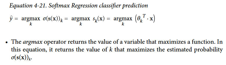
• The idea is quite simple: when given an instance $x$, the Softmax Regression modelfirst computes a score $s_k$$(x)$ for each class $k$, then estimates the probability of eachclass by applying the softmax function (also called the normalized exponential) to thescores. The equation to compute $s_k$$(x)$ should look familiar, as it is just like the equa‐tion for Linear Regression prediction
• Note that each class has its own dedicated parameter vector $θ_k$. All these vectors are typically stored as rows in a parameter matrix $Θ$.
• Once you have computed the score of every class for the instance x, you can estimatethe probability $p_k$ that the instance belongs to class $k$ by running the scores through the softmax function
• Just like the Logistic Regression classifier, the Softmax Regression classifier predicts the class with the highest estimated probability (which is simply the class with thehighest score)
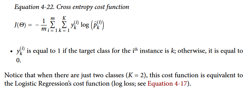
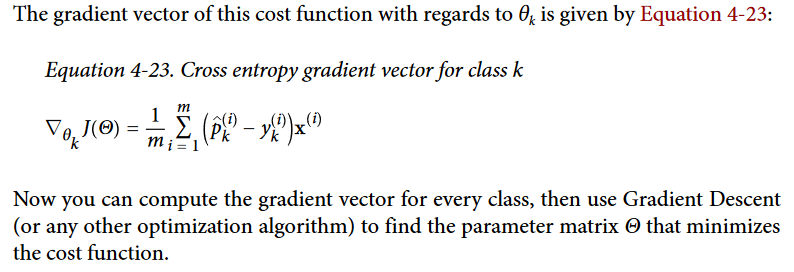
• Cost Function for Softmax Regression

# iris classification using Softmax
X = iris["data"][:, (2, 3)]  # petal length, petal width
y = iris["target"]

softmax_reg = LogisticRegression(multi_class="multinomial",solver="lbfgs", C=10, random_state=42)
softmax_reg.fit(X, y)

LogisticRegression(C=10, class_weight=None, dual=False, fit_intercept=True,
                   intercept_scaling=1, l1_ratio=None, max_iter=100,
                   multi_class='multinomial', n_jobs=None, penalty='l2',
                   random_state=42, solver='lbfgs', tol=0.0001, verbose=0,
                   warm_start=False)

x0, x1 = np.meshgrid(
        np.linspace(0, 8, 500).reshape(-1, 1),
        np.linspace(0, 3.5, 200).reshape(-1, 1),
    )
X_new = np.c_[x0.ravel(), x1.ravel()]


y_proba = softmax_reg.predict_proba(X_new)
y_predict = softmax_reg.predict(X_new)

zz1 = y_proba[:, 1].reshape(x0.shape)
zz = y_predict.reshape(x0.shape)

plt.figure(figsize=(10, 4))
plt.plot(X[y==2, 0], X[y==2, 1], "g^", label="Iris-Virginica")
plt.plot(X[y==1, 0], X[y==1, 1], "bs", label="Iris-Versicolor")
plt.plot(X[y==0, 0], X[y==0, 1], "yo", label="Iris-Setosa")

from matplotlib.colors import ListedColormap
custom_cmap = ListedColormap(['#fafab0','#9898ff','#a0faa0'])

plt.contourf(x0, x1, zz, cmap=custom_cmap)
contour = plt.contour(x0, x1, zz1, cmap=plt.cm.brg)
plt.clabel(contour, inline=1, fontsize=12)
plt.xlabel("Petal length", fontsize=14)
plt.ylabel("Petal width", fontsize=14)
plt.legend(loc="center left", fontsize=14)
plt.axis([0, 7, 0, 3.5])
plt.show()

softmax_reg.predict([[5, 2]])

array([2])

softmax_reg.predict_proba([[5, 2]])

array([[6.38014896e-07, 5.74929995e-02, 9.42506362e-01]])